
2.3 Testing Categorical Data
1 Null hypothesis and testing
They way statistical test work is the following. Assume a hypothesis and answer the question: what is the probability of obtaining the observed result given this hypothesis? This hypothesis is called the null hypothesis and the probability is called p.
In general, the null hypothesis represents a default state of affairs. For example, if we want to compare two samples, the null hypothesis may be that there is no statistical difference between them. The idea is that if there is a difference between the samples, then the probability of observing the observed data will be low.
This brings the question of how low is low enough to establish the difference between samples. There is no definitive answer to this, but the limit p < 0.05, representing a chance of less than 5% of observing this data, is socially considered as good evidence.
2 Which test should I use?
Many statistical tests exist, each with different characteristics and conditions of use. Here we are going to focus on two of the most popular ones: Pearson’s chi-squared test and Fisher’s exact test. In the following, we will use these tests to evaluate the difference between samples.
The difference between these two tests is how well they perform depending on the sample size. Pearson’s chi-squared test has an assumption that is only reasonable when the sample size is big, but it performs well under this constraint. On the other hand, Fisher’s exact test doesn’t depend on the same assumption, and therefore gives better results when sample sizes are small.
Therefore, if you have categorical data to compare, look at your sample size. If you don’t have much data, Fisher’s test is a good first step, otherwise, if you have lots of data, Pearson’s test is good first choice.
3 Fisher’s exact test
Let’s suppose we want to evaluate whether there is a difference in a given population between men and women with relation to studies. The available data is the following (source):
| Men | Women | |
|---|---|---|
| Studying | 1 | 9 |
| Not-studying | 11 | 3 |
In this particular case, we can see there is a large difference between distributions. But how significant is this statistically? To calculate this, we enrich the table with data for each row and column.
| Men | Women | Row total | |
|---|---|---|---|
| Studying | 1 | 9 | 10 |
| Not-studying | 11 | 3 | 14 |
| Column total | 12 | 12 | 24 |
Schematically, we can see this table as this:
| Men | Women | Row Total | |
|---|---|---|---|
| Studying | a | b | a + b |
| Non-studying | c | d | c + d |
| Column Total | a + c | b + d | a + b + c + d (=n) |
Fisher’s exact test says that the probability of observing such data is:
p = \frac{{{{a + b} \choose a}}{{{c + d} \choose c}}}{{n \choose {a + c}}} \qquad{(1)}
where we use the binomial coefficients:
{n \choose m} = \frac{n!}{m!(n-m)!} \qquad{(2)}
So, using eq. 1 and eq. 2 in this particular case we have: p = 0.0013 That is, a chance of 0.13% of observing this data, which is very low and is therefore evidence for the difference between distributions.
In Excel, the binomial coefficients can be calculated using the COMBIN/ЧИСЛКОМБ function.
3.1 Exercise
We will divide the class between men and women, and count the frequencies of total students, and absent students. Then we will see if the distributions are the same or not, using Fisher’s exact test.
4 Pearson’s chi-squared test
One of the most commonly used test to evaluate differences for categorical data is Pearson’s chi-squared test for homogeneity.
4.1 Method
We start with categorical data about two groups A and B, and their occurrences for categories 1 to K.
| Group A (Observed) | Group B (Observed) | |
|---|---|---|
| Category 1 | a1 | b1 |
| Category 2 | a2 | b2 |
| … | … | … |
| Category K | aK | bK |
We then enrich this table with row and column totals.
| Group A (Observed) | Group B (Observed) | Row Total | |
|---|---|---|---|
| Category 1 | a1 | b1 | a1 + b1 = n1 |
| Category 2 | a2 | b2 | a2 + b2 = n2 |
| … | … | … | … |
| Category K | aK | bK | aK + bK = nK |
| Column Total | a1 + … + aK = a | b1 + … + bK = b | a + b = n1 + … + nK = n |
We then replace occurrences with expected frequencies:
| Group A (Expected) | Group B (Expected) | |
|---|---|---|
| Category 1 | a * n1 / n | b * n1 / n |
| Category 2 | a * n2 / n | b * n2 / n |
| … | … | … |
| Category K | a * nK / n | b * nK / n |
Then, for each cell we calculate the chi-square value for each cell, which is:
\chi = \frac{(O - E)^2}{E}
where O is the observed value, and E the expected one, and then sum the values.
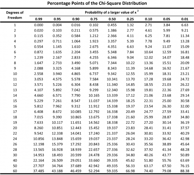
Finally, we need the degrees of freedom. In our case it’s the number of rows minus one, times the number of columns minus one, that is, K - 1.
Then, we use these two values and consult a chi-square values table, such as this one:
4.2 Example
We start with data about how people who live alone or with others eat (source).
| Living Alone | Living With Others | Row Total | |
|---|---|---|---|
| On a diet | 2 | 25 | 27 |
| Pays attention | 23 | 146 | 169 |
| Eats anything | 7 | 124 | 131 |
| Column Total | 32 | 295 | 327 |
We then calculate expected values:
| Living Alone | Living With Others | |
|---|---|---|
| On a diet | 2.6 | 24.4 |
| Pays attention | 16.5 | 152.5 |
| Eats anything | 12.8 | 118.2 |
And then the chi-squared values:
| Living Alone | Living With Others | |
|---|---|---|
| On a diet | 0.138 | 0.0014 |
| Pays attention | 2.560 | 0.277 |
| Eats anything | 1.800 | 1.386 |
The total sum is 5.9 and the degrees of freedom are 2. Consulting the table above, that gives us a p-value a slightly larger than 0.05.
On Excel, we can use the CHISQ.TEST/ХИ2.ТЕСТ function, whose first argument is the observed table, and the second the expected one.
4.3 Exercise
We will use the cancer data and compare observables for people with cancer and without cancer.
5 Control
Take the following data table, and do the following tasks:
- Build the histogram showind the Left/Right distribution for women.
- Build the histogram showind the Left/Right distribution for men.
- Apply Fisher’s test to these two histograms, and calculate the p-value (see the section above).
- Apply Pearson’s chi-squared test to these two histograms, and calculate the p-value. Use the Excel function mentioned in the section above.